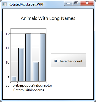
43 rotate axis labels excel 2016
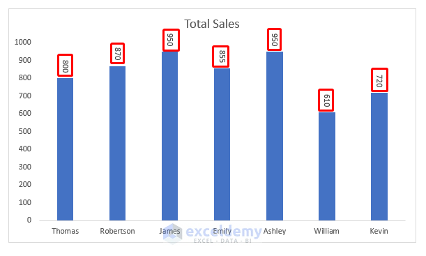
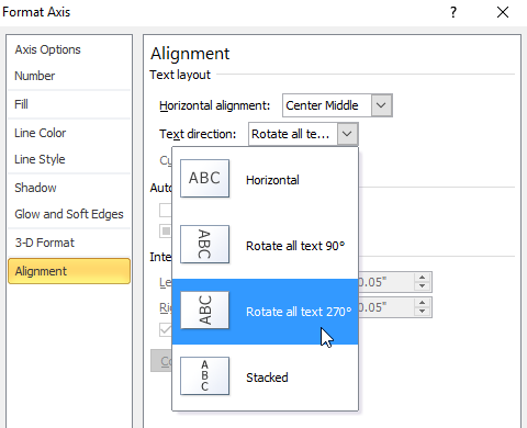
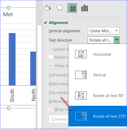
How to Create a Timeline Chart in Excel - Automate Excel This tutorial will demonstrate how to create a timeline chart in all versions of Excel: 2007, 2010, 2013, 2016, and 2019. Timeline Chart – Free Template Download ... Check the “Secondary Axis” box for both of them. Step #5: Add custom data labels. ... rotate the custom data labels 270 degrees to fit them into the columns. Plot One Variable: Frequency Graph, Density Distribution and Nov 17, 2017 · To visualize one variable, the type of graphs to use depends on the type of the variable: For categorical variables (or grouping variables). You can visualize the count of categories using a bar plot or using a pie chart to show the proportion of each category.; For continuous variable, you can visualize the distribution of the variable using density plots, …
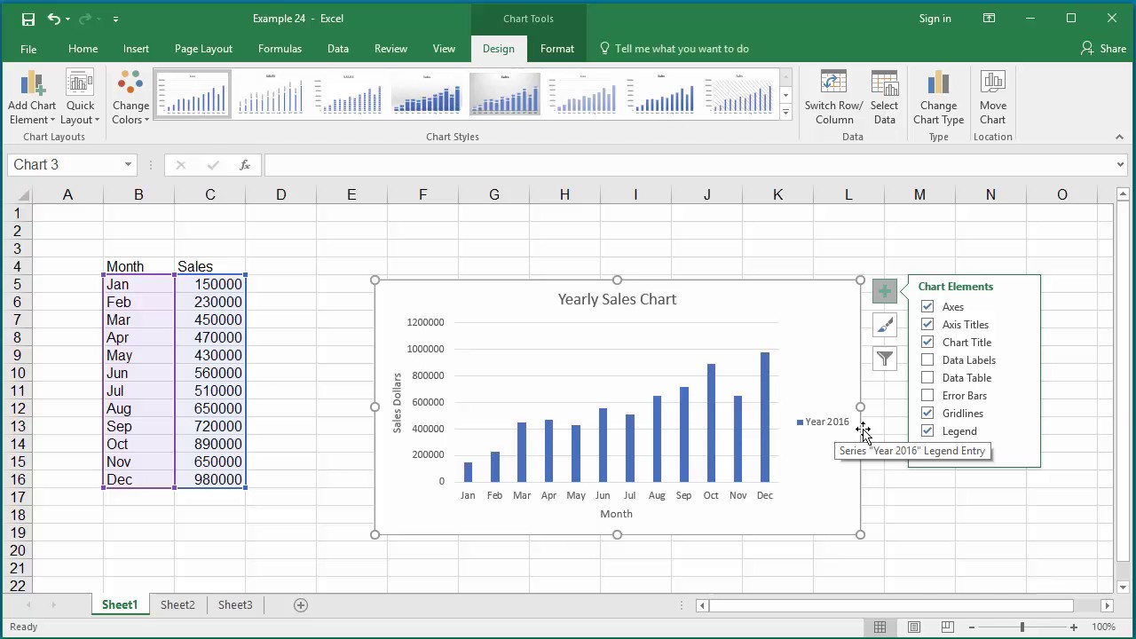
Excel charts: add title, customize chart axis, legend and ... Oct 29, 2015 · For most chart types, the vertical axis (aka value or Y axis) and horizontal axis (aka category or X axis) are added automatically when you make a chart in Excel. You can show or hide chart axes by clicking the Chart Elements button , then clicking the arrow next to Axes , and then checking the boxes for the axes you want to show and unchecking ...

Rotate axis labels excel 2016
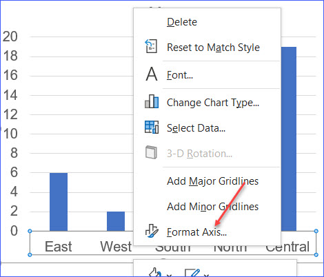
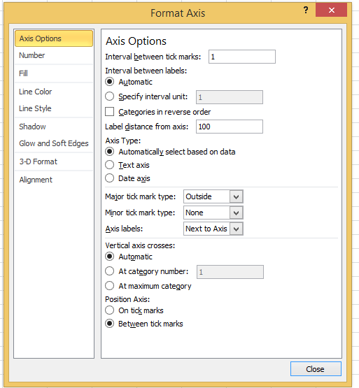
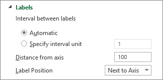
How to Create an Ogive Graph in Excel - Automate Excel Step #6: Change the vertical axis scale. Without closing the pane, jump to the vertical axis (the numbers along the left side) and, by the same token, set the Maximum Bounds value to the total amount of the observations (100). Step #7: Add the data labels. As we proceed to polish the graph, the next logical step is to add the data labels. How to rotate axis labels in chart in Excel? - ExtendOffice 1. Right click at the axis you want to rotate its labels, select Format Axis from the context menu. See screenshot: 2. In the Format Axis dialog, click Alignment tab and go to the Text Layout section to select the direction you need from the list box of Text direction. See screenshot: 3. Close the dialog, then you can see the axis labels are ... Tornado Chart Excel Template – Free Download – How to Create Step #8: Move the category axis labels to the left. Right-click on the vertical category axis labels (in our case, the product names) and choose “Format Axis.” Next, in the “Format Axis” pane, go to the “Axis Options” tab, move down to the “Labels” section, and set the “Label Position” to “Low.
Rotate axis labels excel 2016. Show Months & Years in Charts without Cluttering - Chandoo.org Nov 17, 2010 · So you can just have Product Group & Product Name in 2 columns and when you make a chart, excel groups the labels in axis. 2. Further reduce clutter by unchecking Multi Level Category Labels option. You can make the chart even more crispier by removing lines separating month names. To do this select the axis, press CTRL + 1 (opens format dialog). Rotate a pie chart - support.microsoft.com If you want to rotate another type of chart, such as a bar or column chart, you simply change the chart type to the style that you want. For example, to rotate a column chart, you would change it to a bar chart. Select the chart, click the Chart Tools Design tab, and then click Change Chart Type. See Also. Add a pie chart. Available chart types ... Join LiveJournal Password requirements: 6 to 30 characters long; ASCII characters only (characters found on a standard US keyboard); must contain at least 4 different symbols; How to Create a Stem-and-Leaf Plot in Excel - Automate Excel Step #13: Add the axis titles. Use the axis titles to label both elements of the chart. Select the chart plot. Go to the Design tab. Click “Add Chart Element.” Select “Axis Titles.” Choose “Primary Horizontal” and “Primary Vertical.” As you may see, the axis titles overlap the chart plot.
How to Create a Histogram in Microsoft Excel - How-To Geek Jul 07, 2020 · If you want to create histograms in Excel, you’ll need to use Excel 2016 or later. Earlier versions of Office (Excel 2013 and earlier) lack this feature. ... you can make changes to it by right-clicking your chart axis labels and pressing the “Format Axis” option. Excel will attempt to determine the bins (groupings) to use for your chart ... How to Create a Pareto Chart in Excel – Automate Excel Right-click on the secondary vertical axis (the numbers along the right side) and select “Format Axis.” Once the Format Axis task pane appears, do the following: Go to the Axis Options; Change the Maximum Bounds to “1.” Step #6: Change the gap width of the columns. (PDF) Excel 2016 Bible.pdf | Chandrajoy Sarkar - Academia.edu Excel 2016 Bible.pdf How to Create a Quadrant Chart in Excel – Automate Excel As a final adjustment, add the axis titles to the chart. Select the chart. Go to the Design tab. Choose “Add Chart Element.” Click “Axis Titles.” Pick both “Primary Horizontal” and “Primary Vertical.” Change the axis titles to fit your chart, and you’re all set. And that is how you harness the power of Excel quadrant charts!
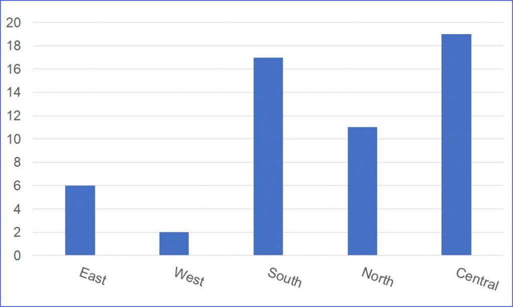
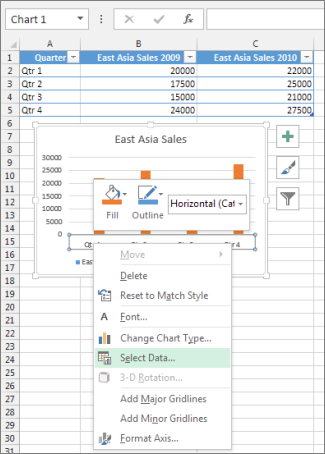
How to create a chart in Excel from multiple sheets - Ablebits.com Sep 29, 2022 · Click on the chart you've just created to activate the Chart Tools tabs on the Excel ribbon, go to the Design tab (Chart Design in Excel 365), and click the Select Data button. Or, click the Chart Filters button on the right of the graph, and then click the … Tornado Chart Excel Template – Free Download – How to Create Step #8: Move the category axis labels to the left. Right-click on the vertical category axis labels (in our case, the product names) and choose “Format Axis.” Next, in the “Format Axis” pane, go to the “Axis Options” tab, move down to the “Labels” section, and set the “Label Position” to “Low. How to rotate axis labels in chart in Excel? - ExtendOffice 1. Right click at the axis you want to rotate its labels, select Format Axis from the context menu. See screenshot: 2. In the Format Axis dialog, click Alignment tab and go to the Text Layout section to select the direction you need from the list box of Text direction. See screenshot: 3. Close the dialog, then you can see the axis labels are ... How to Create an Ogive Graph in Excel - Automate Excel Step #6: Change the vertical axis scale. Without closing the pane, jump to the vertical axis (the numbers along the left side) and, by the same token, set the Maximum Bounds value to the total amount of the observations (100). Step #7: Add the data labels. As we proceed to polish the graph, the next logical step is to add the data labels.
How to Rotate Axis Labels in Origin | TUTORIAL

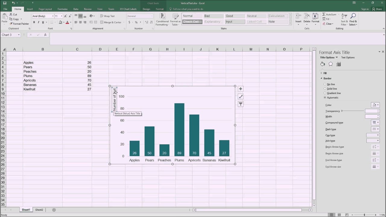
Microsoft Excel Tutorials: Format Axis Titles
Turn your head and check out this post [How to: Easily rotate ...
How to Change Elements of a Chart like Title, Axis Titles, Legend etc in Excel 2016
Customize C# Chart Options - Axis, Labels, Grouping ...
How to Rotate X Axis Labels in Chart - ExcelNotes

Two-Level Axis Labels (Microsoft Excel)
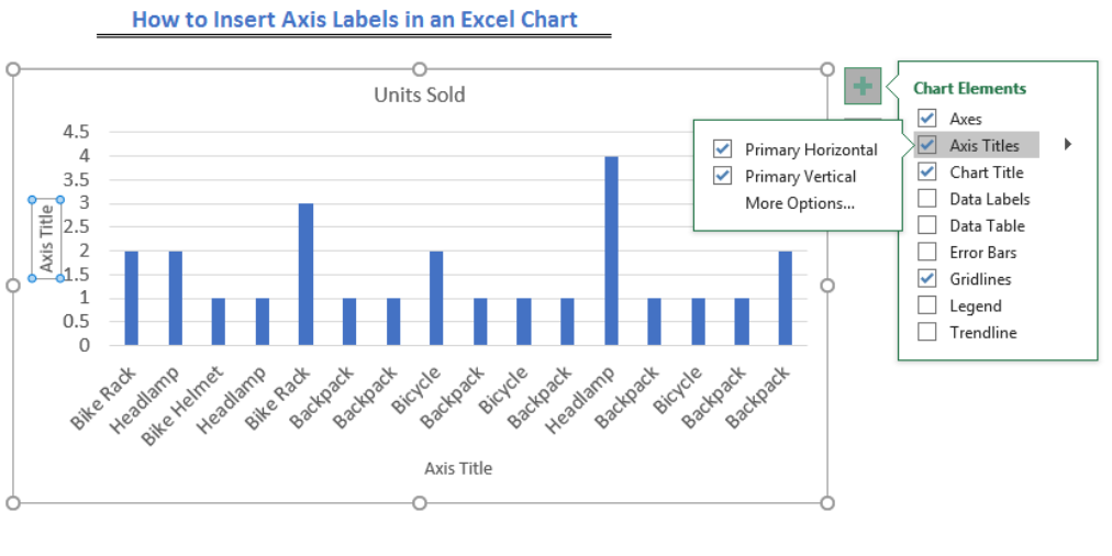
How to Insert Axis Labels In An Excel Chart | Excelchat

Excel charts: add title, customize chart axis, legend and ...
Adding horizontally-aligned y-axis titles to charts in Excel 2016
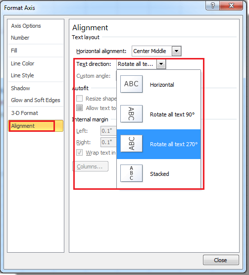
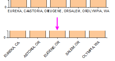
How to rotate axis labels in chart in Excel?
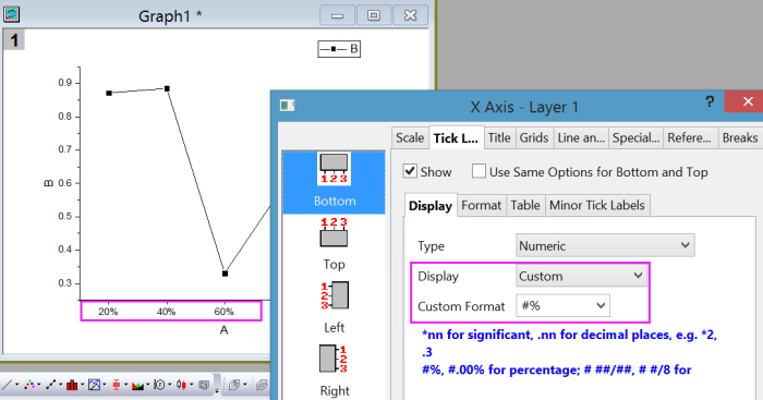
Help Online - Quick Help - FAQ-121 What can I do if my tick ...

Changing Axis Labels in PowerPoint 2013 for Windows
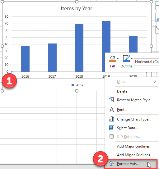
Change axis labels in a chart in Office

Change axis labels in a chart in Office
Rotate a Chart in Excel & Google Sheets - Automate Excel
How to Rotate Data Labels in Excel (2 Simple Methods)
Rotate Chart Axis Category Labels Vertical 270 degrees ...
How to Rotate X Axis Labels in Chart - ExcelNotes

Add or remove titles in a chart

How do I resize the text axis box of a graph in Excel 2016 ...

How to wrap X axis labels in a chart in Excel?

How to add axis labels in excel | WPS Office Academy
How to Rotate X Axis Labels in Chart - ExcelNotes

How to Label Axes in Excel: 6 Steps (with Pictures) - wikiHow
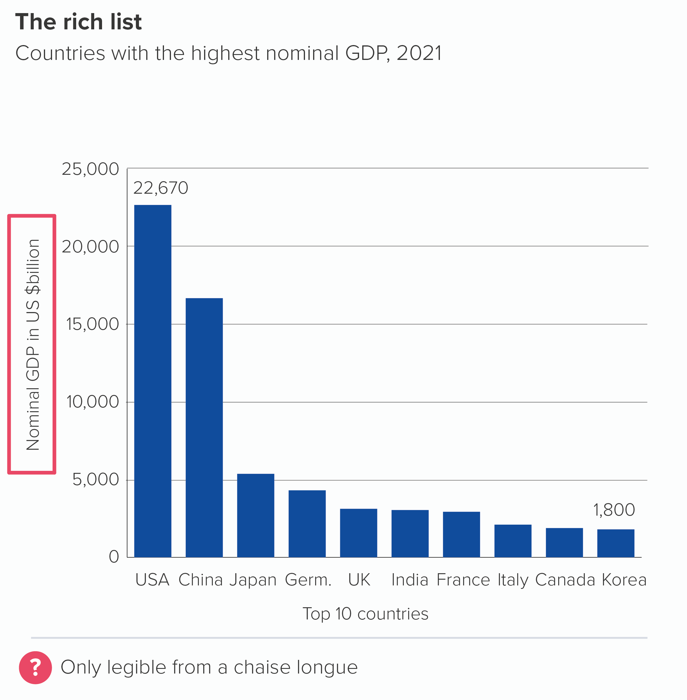
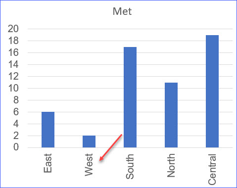
Rule 24: Label your bars and axes — AddTwo
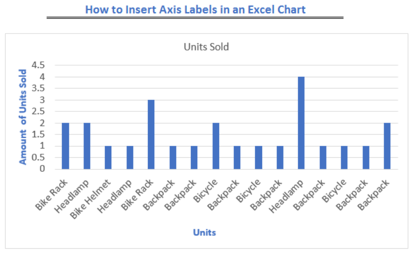
How to Insert Axis Labels In An Excel Chart | Excelchat
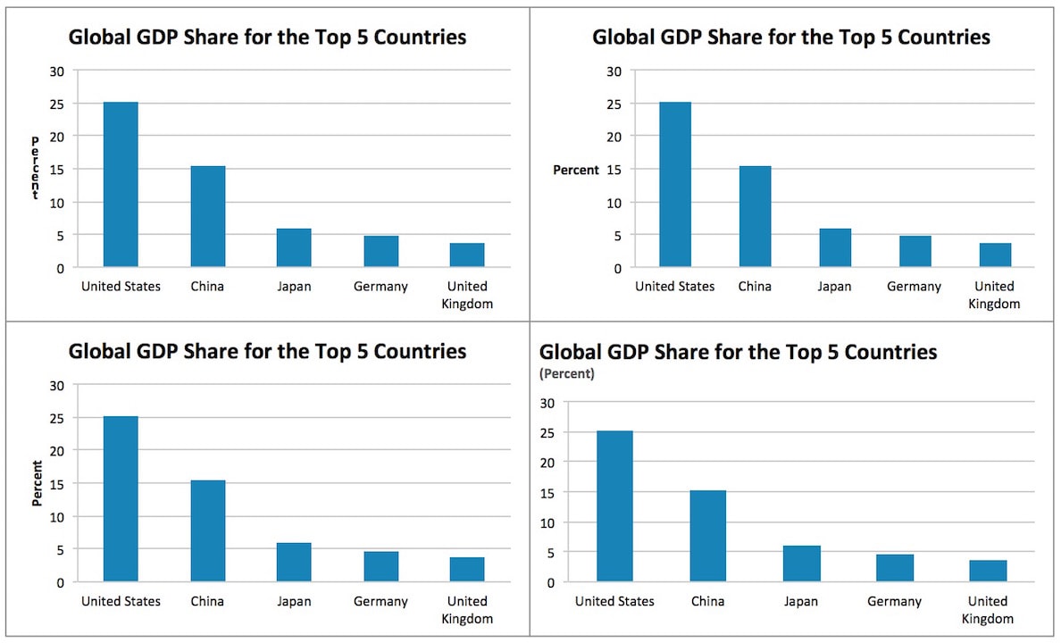
Where to Position the Y-Axis Label - PolicyViz
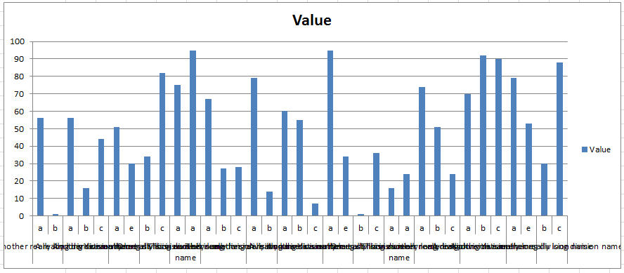
3 Ways to Make Excel Chart Horizontal Categories Fit Better ...
How to Rotate X Axis Labels in Chart - ExcelNotes
Change axis labels in a chart

charts - How do I create custom axes in Excel? - Super User

Rule 24: Label your bars and axes — AddTwo
Help Online - Quick Help - FAQ-122 How do I format the axis ...
Rotate a Chart in Excel & Google Sheets - Automate Excel

Microsoft Excel Tutorials: Format Axis Titles
Where to Position the Y-Axis Label - PolicyViz
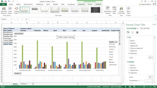
How to Customize Your Excel Pivot Chart and Axis Titles - dummies

How to Change Orientation of Multi-Level Labels in a Vertical ...
How to move Y axis to left/right/middle in Excel chart?
Change the display of chart axes
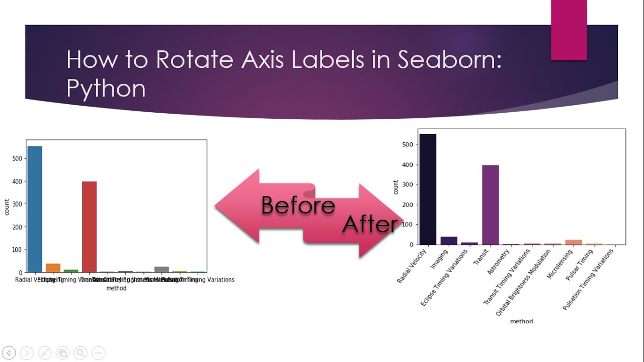
How to rotate axis labels in Seaborn | Python Machine Learning
Excel Chart Vertical Axis Text Labels • My Online Training Hub
Post a Comment for "43 rotate axis labels excel 2016"