38 format data labels pane excel

How do you format data series in Excel? - faq-all.com To format data labels in EÎl , choose the set of data labels to format . To do this, click the " Format " tab within the "Chart Tools" contextual tab in the Ribbon. Then select the data labels to format from the "Chart Elements" drop-down in the "Current Selection" button group. How do I show the Format Data Series pane in Excel? PDF Where is the format data labels task pane in excel Where is the format data labels task pane in excel ... In Excel 2013's Format Axis pane, expand the Number group on the Axis Options tab, click the Category box and select Number from drop down list, and then click to select a red Negative number style in the Negative numbers box. (2) In Excel 2007 and 2010's Format Axis dialog box, click ...

Excel Charts - Aesthetic Data Labels - tutorialspoint.com To format the data labels − Step 1 − Right-click a data label and then click Format Data Label. The Format Pane - Format Data Label appears. Step 2 − Click the Fill & Line icon. The options for Fill and Line appear below it. Step 3 − Under FILL, Click Solid Fill and choose the color.

Format data labels pane excel

How to Customize Your Excel Pivot Chart Data Labels - dummies To remove the labels, select the None command. If you want to specify what Excel should use for the data label, choose the More Data Labels Options command from the Data Labels menu. Excel displays the Format Data Labels pane. Check the box that corresponds to the bit of pivot table or Excel table information that you want to use as the label. How to Create Mailing Labels in Excel | Excelchat Step 1 - Prepare Address list for making labels in Excel First, we will enter the headings for our list in the manner as seen below. First Name Last Name Street Address City State ZIP Code Figure 2 - Headers for mail merge Tip: Rather than create a single name column, split into small pieces for title, first name, middle name, last name. Add a DATA LABEL to ONE POINT on a chart in Excel You can now configure the label as required — select the content of the label (e.g. series name, category name, value, leader line), the position (right, left, above, below) in the Format Data Label pane/dialog box. To format the font, color and size of the label, now right-click on the label and select 'Font'. Note: in step 5. above, if ...

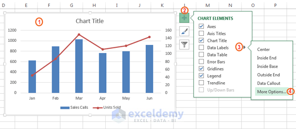
Format data labels pane excel. Format Data Label: Label Position - Microsoft Community when you add labels with the + button next to the chart, you can set the label position. In a stacked column chart the options look like this: For a clustered column chart, there is an additional option for "Outside End" When you select the labels and open the formatting pane, the label position is in the series format section. Does that help? How to Print Labels from Excel - Lifewire Navigate to the Excel worksheet containing your list in the Select Data Source window that opens and click Open . Click OK to confirm that you want to use the list and click OK again to select the table containing your list. The page will now be filled with labels that say « Next Record» . Add Mail Merge Fields and Perform the Merge 1/ Select A1:B7 > Inser your Histo. chart. 2/ Right-click i.e. on the 1st histo. bar (A) > Add Data Labels (numbers are displayed a the top of the bars) 3/ Click one of the numbers that just displayed (the Format Data Labels pane opens on the right) > Check option "Value From Cells" > Select range C2:C7 > OK > Uncheck option "Value". Adding rich data labels to charts in Excel 2013 | Microsoft 365 Blog Putting a data label into a shape can add another type of visual emphasis. To add a data label in a shape, select the data point of interest, then right-click it to pull up the context menu. Click Add Data Label, then click Add Data Callout . The result is that your data label will appear in a graphical callout.

Pie Chart in Excel - Inserting, Formatting, Filters, Data Labels Click on the Instagram slice of the pie chart to select the instagram. Go to format tab. (optional step) In the Current Selection group, choose data series "hours". This will select all the slices of pie chart. Click on Format Selection Button. As a result, the Format Data Point pane opens. Custom Chart Data Labels In Excel With Formulas - How To Excel At Excel Select the chart label you want to change. In the formula-bar hit = (equals), select the cell reference containing your chart label's data. In this case, the first label is in cell E2. Finally, repeat for all your chart laebls. If you are looking for a way to add custom data labels on your Excel chart, then this blog post is perfect for you. Formatting data labels and printing pie charts on Excel for Mac 2019 ... Still can't find a solution for formatting the data labels. 1. When printing a pie chart from Excel for mac 2019, MS instructions are to select the chart only, on the worksheet > file > print. Excel is supposed to print the chart only (not the data ) and automatically fit it onto one page. This doesn't work on my machine. Advanced Excel - Richer Data Labels - tutorialspoint.com We use a Bubble Chart to see the formatting of Data Labels. Step 1 − Select your data. Step 2 − Click on the Insert Scatter or the Bubble Chart. The options for the Scatter Charts and the 2-D and 3-D Bubble Charts appear. Step 3 − Click on the 3-D Bubble Chart. The 3-D Bubble Chart will appear as shown in the image given below.

Excel 2016 Tutorial Formatting Data Labels Microsoft Training Lesson Click: Learn about Formatting Data Labels in Microsoft Excel at . A clip from Mastering Excel Made Easy v. 2016. Format Data Labels in Excel- Instructions - TeachUcomp, Inc. Format Data Labels in Excel: Instructions To format data labels in Excel, choose the set of data labels to format. One way to do this is to click the "Format" tab within the "Chart Tools" contextual tab in the Ribbon. Then select the data labels to format from the "Current Selection" button group. ... Excel 2019 & 365 Tutorial Formatting Data Labels Microsoft Training Click: Learn about Formatting Data Labels in Microsoft Excel at . How to Display the Format Data Labels Task Pane Change the chart title. Analyze Data in Excel will analyze your data and return interesting visuals about it in a task pane. In the Cloud console select Monitoring. Move the labels to the appropriate places above the gauge chart. Using either method then displays the Format Data Labels task pane at the right side of the screen.

Format Data Labels in Excel- Instructions - TeachUcomp, Inc.

Excel tutorial: The Format Task pane You can select element, and then click the Format Selection button on the Chart Tools Format tab, or, easier, right-click any element and choose the format option from the shortcut menu. Notice when you right-click a chart element, you'll see a shortcut menu and something called the mini-toolbar, which provides quick access to common formatting tasks, plus a small menu to browse and select chart elements. The content in the Format Task Pane varies a lot depending on what element is selected.

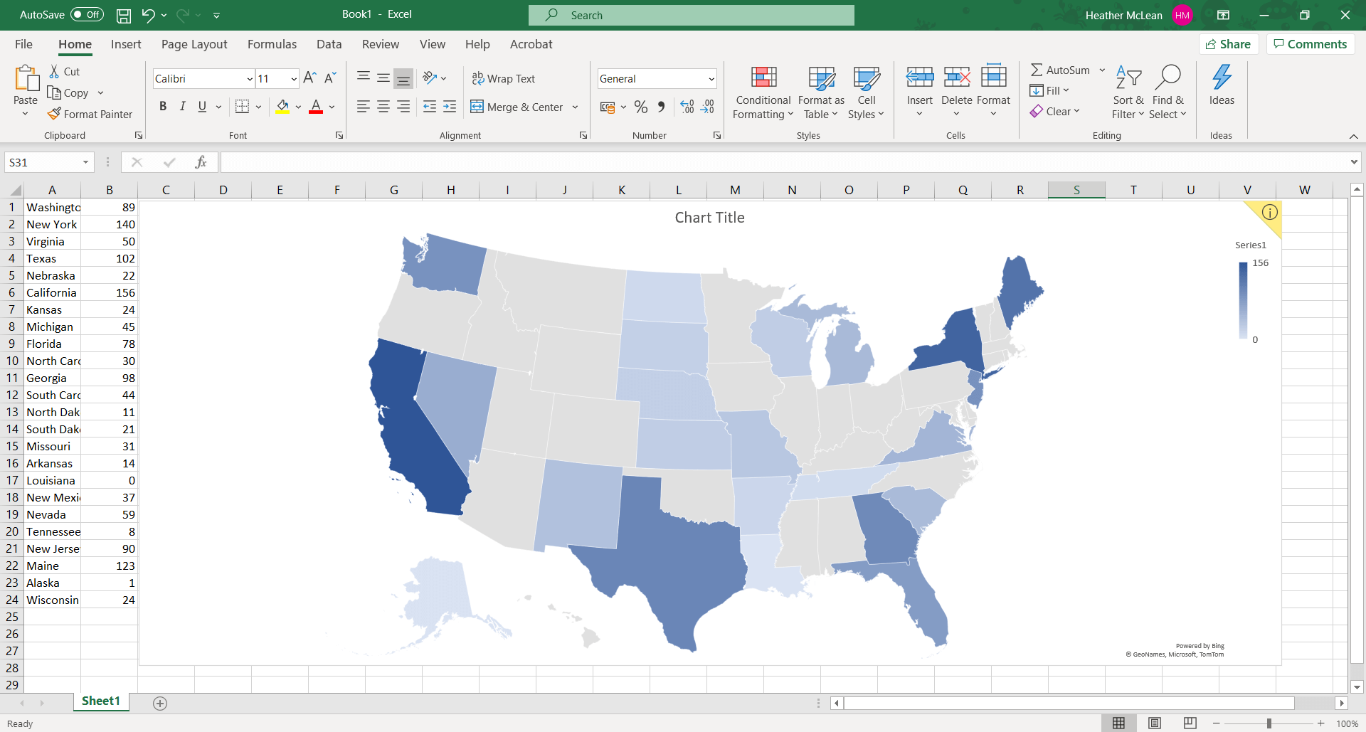
Geographical heat map: Excel vs eSpatial - eSpatial

How to Print Labels From Excel - EDUCBA You can download this How to Print Labels From Excel Template here - How to Print Labels From Excel Template Step #1 - Add Data into Excel Create a new excel file with the name "Print Labels from Excel" and open it. Add the details to that sheet. As we want to create mailing labels, make sure each column is dedicated to each label. Ex.

Microsoft Excel Tutorials: The Chart Layout Panels

How To Format Data Labels In Excel - Walls Alawavell At that place are many options available for formatting of the Data Label in the Format Data Labels Task Pane. Brand sure that only one Information Label is selected while formatting. Stride 9 − In Characterization Options → Data Label Series, click on Clone Current Label.

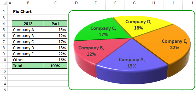
How to show percentage in pie chart in Excel?

How to format axis labels as thousands/millions in Excel? - ExtendOffice 1. Right click at the axis you want to format its labels as thousands/millions, select Format Axis in the context menu. 2. In the Format Axis dialog/pane, click Number tab, then in the Category list box, select Custom, and type [>999999] #,,"M";#,"K" into Format Code text box, and click Add button to add it to Type list. See screenshot: 3.

Apply Custom Data Labels to Charted Points - Peltier Tech Blog

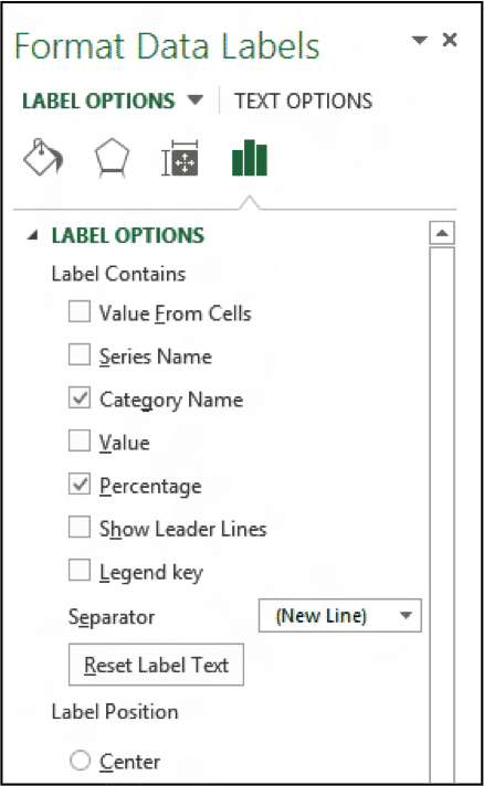
Excel tutorial: How to use data labels In a bar or column chart, data labels will first appear outside the bar end. You'll also find options for center, inside end, and inside base. There's also a feature called "data callouts" which wraps data labels in a shape. When first enabled, data labels will show only values, but the Label Options area in the format task pane offers many other settings. You can set data labels to show the category name, the series name, and even values from cells.

Add or remove data labels in a chart - Office Support

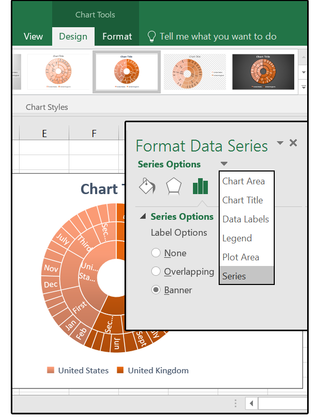
Format elements of a chart - support.microsoft.com Format your chart using the Format task pane. Select the chart element (for example, data series, axes, or titles), right-click it, and click Format . The Format pane appears with options that are tailored for the selected chart element. Clicking the small icons at the top of the pane moves you to other parts of the pane with more options.

Excel 3-D Pie charts - Microsoft Excel 2013

Change the format of data labels in a chart To format data labels, select your chart, and then in the Chart Design tab, click Add Chart Element > Data Labels > More Data Label Options. Click Label Options and under Label Contains , pick the options you want.

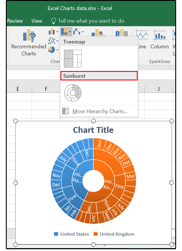
What to do with Excel 2016's new chart styles: Treemap, Sunburst, and Box & Whisker | PCWorld

How to add data labels from different column in an Excel chart? Right click the data series, and select Format Data Labels from the context menu. 3. In the Format Data Labels pane, under Label Options tab, check the Value From Cells option, select the specified column in the popping out dialog, and click the OK button. Now the cell values are added before original data labels in bulk. 4.

What to do with Excel 2016's new chart styles: Treemap, Sunburst, and Box & Whisker | PCWorld

Add a DATA LABEL to ONE POINT on a chart in Excel You can now configure the label as required — select the content of the label (e.g. series name, category name, value, leader line), the position (right, left, above, below) in the Format Data Label pane/dialog box. To format the font, color and size of the label, now right-click on the label and select 'Font'. Note: in step 5. above, if ...

Change the format of data labels in a chart - Office Support

How to Create Mailing Labels in Excel | Excelchat Step 1 - Prepare Address list for making labels in Excel First, we will enter the headings for our list in the manner as seen below. First Name Last Name Street Address City State ZIP Code Figure 2 - Headers for mail merge Tip: Rather than create a single name column, split into small pieces for title, first name, middle name, last name.